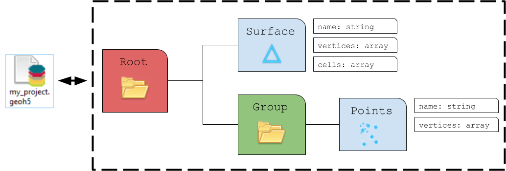
Objects

The geoh5 format enables storing a wide variety of Object entities that can be displayed in 3D. This section describes the collection of Objects entities currently supported by geoh5py.

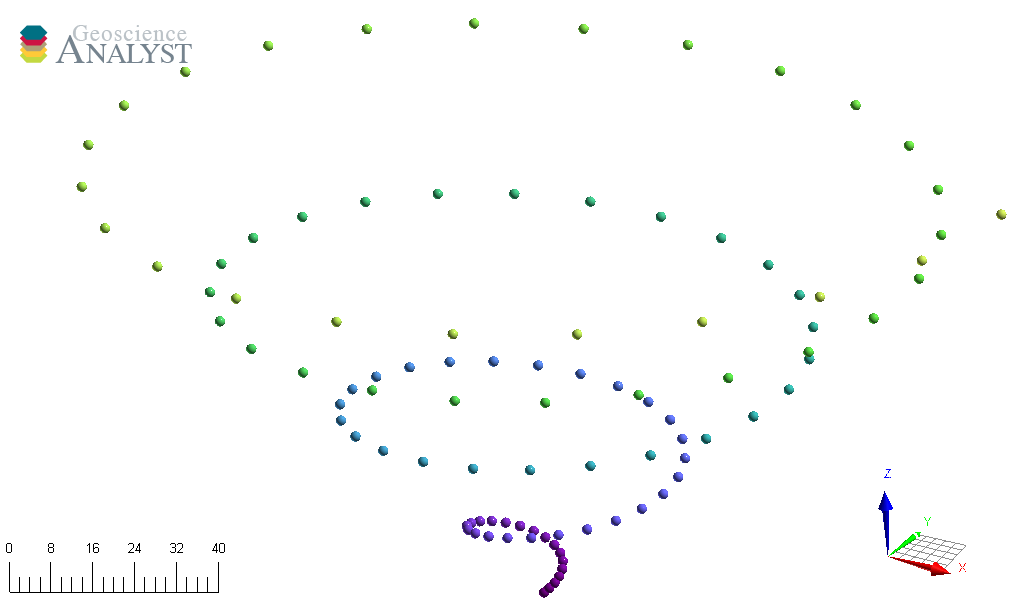
Points

The Points object consists of a list of vertices that define the location of actual data in 3D space. As for all other Objects, it can be created from an array of 3D coordinates and added to any group as follow:

import numpy as np

from geoh5py import Workspace
from geoh5py.objects import Points


# Get a project
with Workspace.create("my_points.geoh5") as workspace:
    # Generate a numpy array of xyz locations
    n = 100
    radius, theta = np.arange(n), np.linspace(0, np.pi * 8, n)

    x, y = radius * np.cos(theta), radius * np.sin(theta)
    z = (x**2.0 + y**2.0) ** 0.5
    xyz = np.c_[x.ravel(), y.ravel(), z.ravel()]  # Form a 2D array

    # Create the Point object
    points = Points.create(
        workspace,  # The target Workspace
        vertices=xyz,  # Set vertices
    )

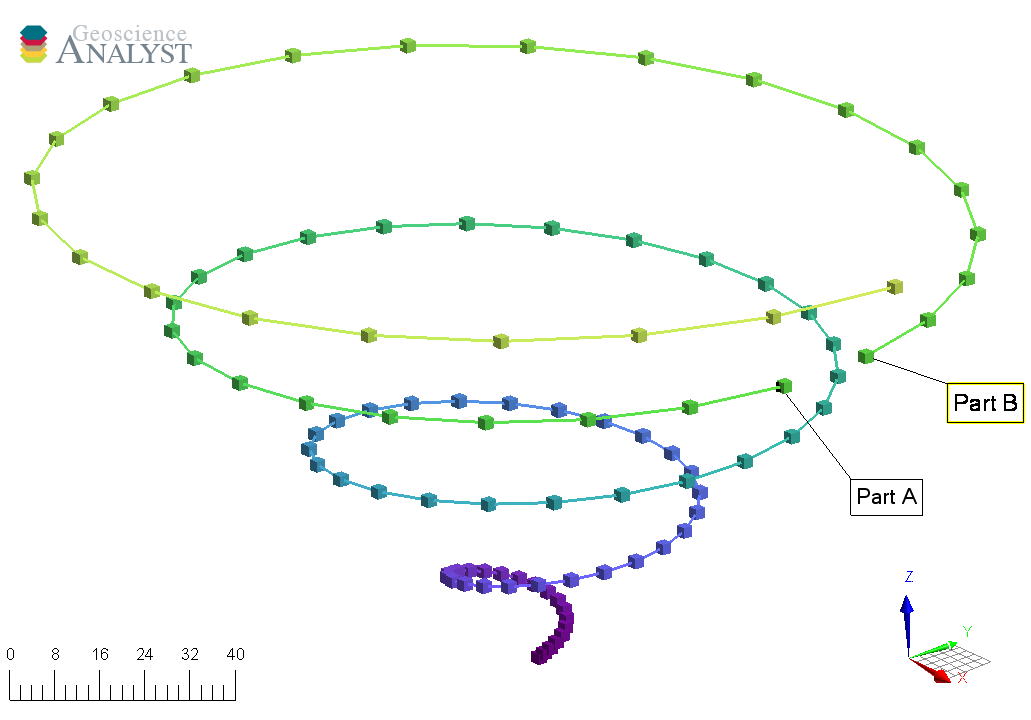
Curve

The Curve object, also known as a polyline, is often used to define contours, survey lines or geological contacts. It is a sub-class of the Points object with the added cells property, that defines the line segments connecting its vertices. By default, all vertices are connected sequentially following the order of the input vertices. A parts identifier may be added to curve objects to distinguish different sections of the curve. This can be useful, for example, in representing a geophysical survey over many lines.

from geoh5py.objects import Curve


# Get a project
with Workspace.create("my_curve.geoh5") as workspace:
    # Split the curve into two parts
    part_id = np.ones(n, dtype="int32")
    part_id[:75] = 2

    # Create the Curve object
    curve = Curve.create(
        workspace,  # The target Workspace
        vertices=xyz,
        parts=part_id,
    )

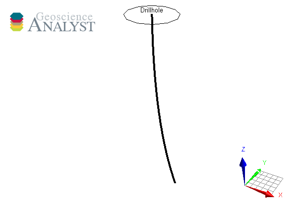
Drillhole

Drillhole objects are different from other objects as their 3D geometry is defined by the collar and surveys attributes. As for version geoh5 v2.0, the drillholes require a DrillholeGroup entity to store the geometry and data.

from geoh5py.groups import DrillholeGroup
from geoh5py.objects import Drillhole


# Get a project
with Workspace.create("my_drillhole.geoh5") as workspace:
    dh_group = DrillholeGroup.create(workspace)

    # Create a simple well
    total_depth = 100
    dist = np.linspace(0, total_depth, 10)
    azm = np.ones_like(dist) * 45.0
    dip = np.linspace(-89, -75, dist.shape[0])
    collar = np.r_[0.0, 10.0, 10]

    well = Drillhole.create(
        workspace,
        collar=collar,
        surveys=np.c_[dist, azm, dip],
        name="Drillhole",
        parent=dh_group,
    )

    print(well.name)

Drillhole

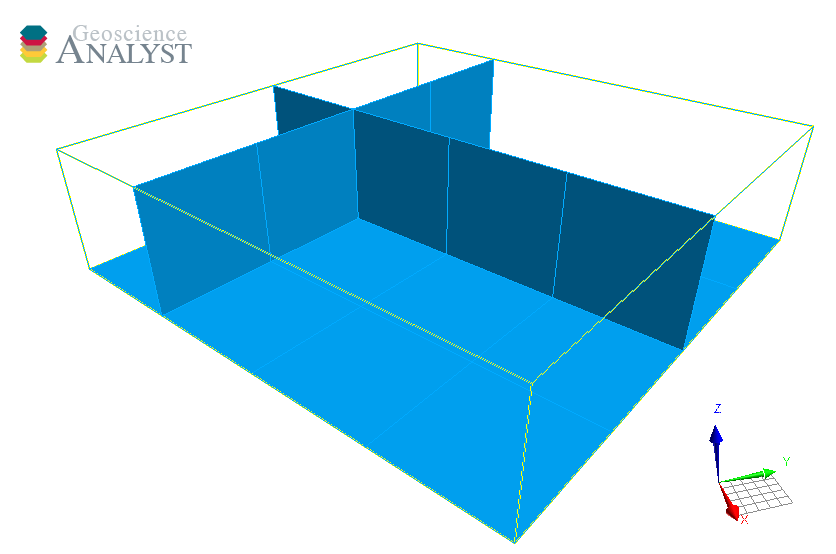
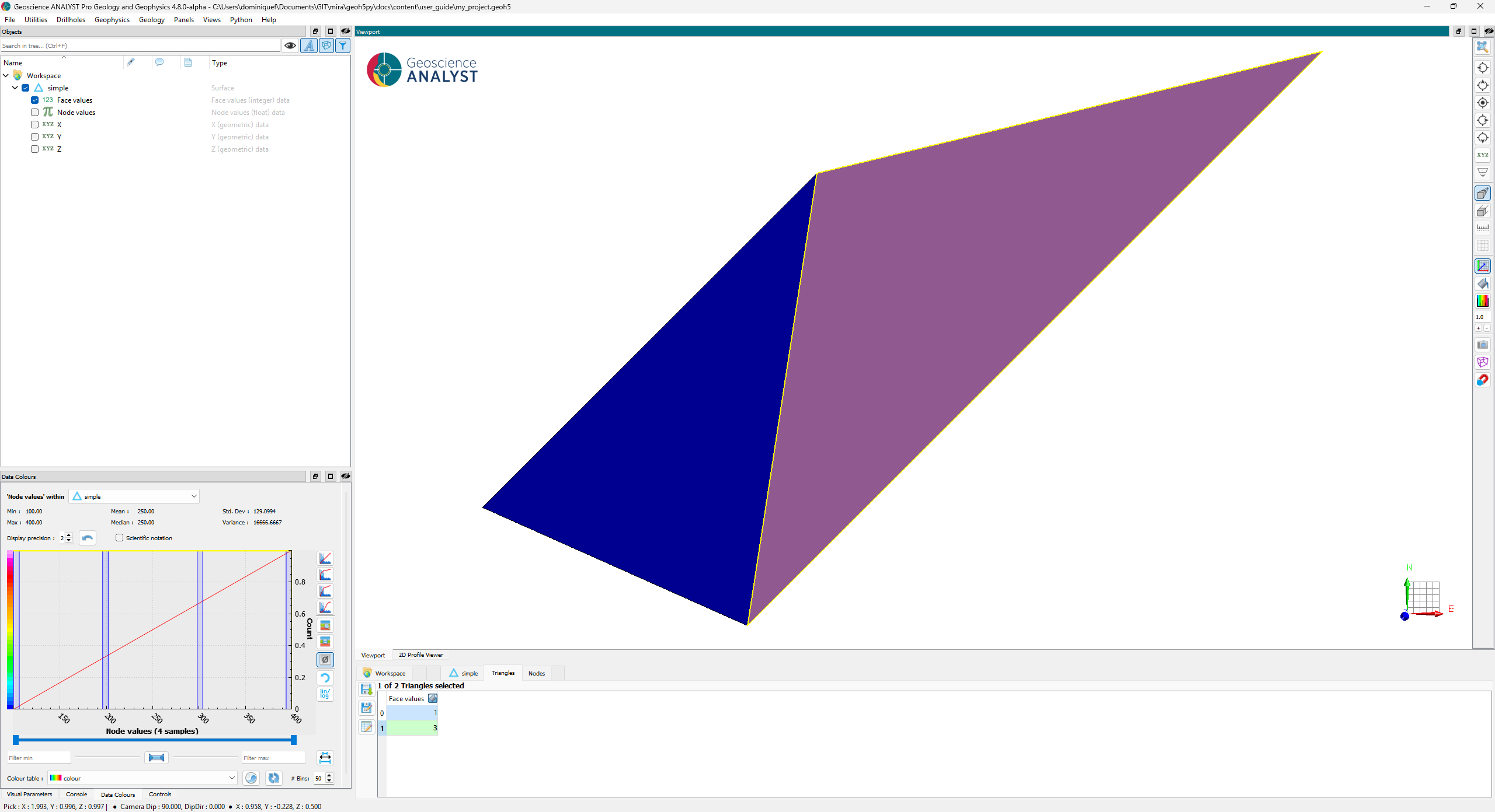
Surface

The Surface object is also described by vertices and cells, which form a net of triangles.

A simple example is shown below.

# Simple example with 4 nodes
vertices = np.array([[0, 0, 0], [1, 0, 1], [1, 1, 0], [2, 1, 1]])

# Array of indices is used to define triangles.
# The order of the nodes determines the direction of the
# normal by the right-hand rule
simplices = np.array([[0, 1, 2], [1, 2, 3]])

We can now add the geometry and some data to geoh5.

from geoh5py.objects import Surface


# Get a project
with Workspace.create("simple_surface.geoh5") as workspace:
    # Create the surface
    surface = Surface.create(
        workspace, vertices=vertices, cells=simplices, name="simple"
    )

    # Data can be added to either the triangles or the nodes.
    # The association can be specified by the user, or determined
    # by the length of the array provided.
    vertex_data_values = np.array([200.0, 100.0, 300.0, 400.0])
    cell_data = surface.add_data(
        {
            "Node values": {  # Name of the data property
                "association": "VERTEX",  # Data associated with vertices
                "values": vertex_data_values,
                "units": "m/s",
            },
            "Face values": {  # Name of the data property
                "values": np.r_[1, 3],  # Two values will be detected as "cell" data.
                "units": "SI",
            },
        }
    )

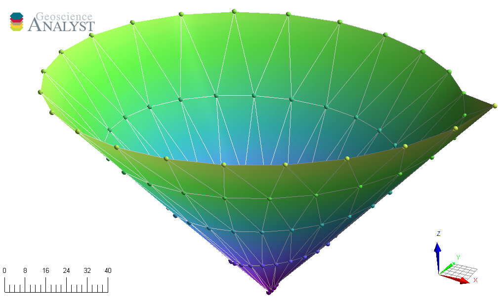
The example below shows how to leverage the scipy.spatial.Delaunay triangulation to build mode complex surfaces.

from scipy.spatial import Delaunay


# Get a project
with Workspace.create("delaunay_surface.geoh5") as workspace:
    # Create a triangulated surface from points
    surf_2D = Delaunay(xyz[:, :2])

    # Create the Surface object
    surface = Surface.create(
        workspace,
        vertices=points.vertices,  # Add vertices
        cells=surf_2D.simplices,
    )

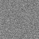
GeoImage

The GeoImage object handles raster data, either single or 3-band images.

from geoh5py.objects import GeoImage


# Get a project
workspace = Workspace.create("my_images.geoh5")
geoimage = GeoImage.create(workspace)

Image values can be assigned to the object from either a 2D numpy.ndarray for single band (gray):

geoimage.image = np.random.randn(128, 128)
display(geoimage.image)

or as 3D numpy.ndarray for 3-band RGB image:

geoimage = GeoImage.create(workspace, image=np.random.randn(128, 128, 3))
display(geoimage.image)

The object can easily be saved back out to file with.

geoimage.save_as("my_image.jpg")

A GeoImage can also be created directly from file (png, jpeg, tiff).

geoimage = GeoImage.create(workspace, image="my_image.jpg")

A PIL.Image object gets exposed to the user, which can be used for common raster manipulation (rotation, filtering, etc). The modified raster is stored back on file as a blob (bytes).

display(geoimage.image)

Geo-referencing

By default, the GeoImage object will be displayed at the origin (xy-plane) with dimensions equal to the pixel count. The utility function GeoImage.georeference lets users geo-reference the image in 3D space based on at least three (3) input reference points (pixels) with associated world coordinates.

pixels = [
    [18, 73, 0],
    [757, 1014, 0],
    [18, 1014, 0],
]
coords = [[311005, 6065252, 0], [320001, 6076748, 0], [311005, 6076748, 0]]

# First, re-arrange the tie points in pairs of coordinates (row-wise).
pairs = np.hstack([np.vstack(pixels), np.vstack(coords)])
# Reshape as 3D array of pairs
pairs = pairs.reshape((-1, 2, 3))

geoimage.georeference(pairs)
print(geoimage.vertices)
workspace.close()

[[ 310785.88227334 6064360.17428268       0.        ]
 [ 312344.05277402 6064360.17428268       0.        ]
 [ 312344.05277402 6065923.92348565       0.        ]
 [ 310785.88227334 6065923.92348565       0.        ]]

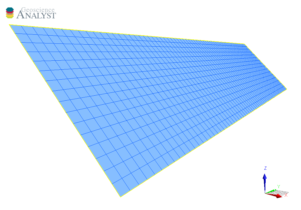
Grid2D

The Grid2D object defines a regular grid of cells often used to display model sections or to compute data derivatives. A Grid2D can be oriented in 3D space using the origin, rotation and dip parameters.

from geoh5py.objects import Grid2D


with Workspace.create("my_grid2d.geoh5") as workspace:
    # Create the Surface object
    grid = Grid2D.create(
        workspace,
        origin=[25, -75, 50],
        u_cell_size=2.5,
        v_cell_size=2.5,
        u_count=64,
        v_count=16,
        rotation=90.0,
        dip=45.0,
    )

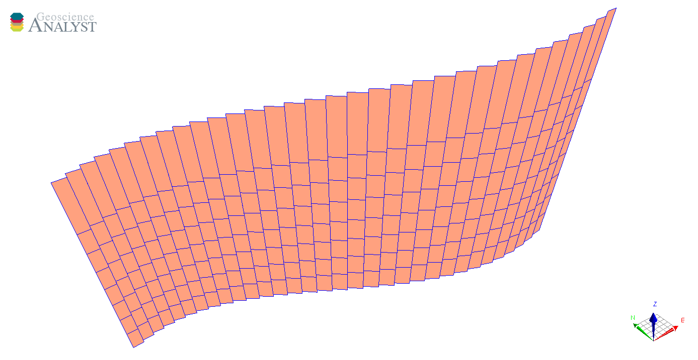
DrapeModel

The DrapeModel object defines an array of vertical (curtain) cells draped below a curved trace.

• The prisms attribute defines the elevation and position of the uppermost cell faces.

• The layers attribute defines the bottom face elevation of cells.

In the example below we create a simple DrapeModel object along a sinusoidal path with equal number of layers below every station. Variable number of layers per prism is also supported.

from geoh5py.objects import DrapeModel


with Workspace.create("my_drape_model.geoh5") as workspace:
    # Define a simple trace
    n_columns = 32
    n_layers = 8

    x = np.linspace(0, np.pi, n_columns)
    y = np.cos(x)
    z = np.linspace(0, 1, n_columns)

    # Count the index and number of values per columns
    layer_count = np.ones(n_columns) * n_layers
    prisms = np.c_[x, y, z, np.cumsum(layer_count) - n_layers, layer_count]

    # Define the index and elevation of draped cells
    k_index, i_index = np.meshgrid(np.arange(n_layers), np.arange(n_columns))
    z_elevation = z[i_index] - np.linspace(0.5, 2, n_layers)

    layers = np.c_[i_index.flatten(), k_index.flatten(), z_elevation.flatten()]

    # Create the object
    drape = DrapeModel.create(workspace, prisms=prisms, layers=layers)

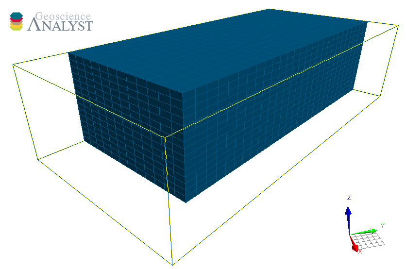
BlockModel

The BlockModel object defines a rectilinear grid of cells, also known as a tensor mesh. The cells center position is determined by cell_delimiters (offsets) along perpendicular axes (u, v, z) and relative to the origin. BlockModel can be oriented horizontally by controlling the rotation parameter.

from geoh5py.objects import BlockModel


with Workspace.create("my_block_model.geoh5") as workspace:
    mesh = BlockModel.create(
        workspace,
        origin=[25, -100, 50],
        u_cell_delimiters=np.cumsum(np.ones(16) * 5),  # Offsets along u
        v_cell_delimiters=np.cumsum(np.ones(32) * 5),  # Offsets along v
        z_cell_delimiters=np.cumsum(np.ones(16) * -2.5),  # Offsets along z (down)
        rotation=30.0,
    )

Data values stored on the BlockModel object, such as centroid coordinates, are stored in [w, u, v] Fortran ordering. The 1D arrays can be resorted as 3D arrays with

x = mesh.centroids[:, 0]
array = x.reshape((mesh.shape[2], mesh.shape[0], mesh.shape[1]), order="F")
print(array.shape)

(15, 15, 31)

The 3D array can be flatten back to 1D with

array.flatten(order="F")

array([27.74519053, 27.74519053, 27.74519053, ..., 13.36696879,
       13.36696879, 13.36696879], shape=(6975,))

Octree

The Octree object is type of 3D grid that uses a tree structure to define cells. Each cell can be subdivided it into eight octants allowing for a more efficient local refinement of the mesh. The Octree object can also be oriented horizontally by controlling the rotation parameter.

from geoh5py.objects import Octree


with Workspace.create("my_octree.geoh5") as workspace:
    octree = Octree.create(
        workspace,
        origin=[25, -100, 50],
        u_count=16,  # Number of cells in power 2
        v_count=32,
        w_count=16,
        u_cell_size=5.0,  # Base cell size (highest octree level)
        v_cell_size=5.0,
        w_cell_size=2.5,  # Offsets along z (down)
        rotation=30,
    )

By default, the octree mesh will be refined at the lowest level possible along each axes.